
Info: Machine translation This post was machine-translated from the Chinese original. Wording may be rough in places — the Chinese version is authoritative.
Summary Give the machine four sets of numbers, don’t tell it patterns, yet it can turn two knobs toward the answer. Now look at the curves in the neuron melting pot: loss decreases, interfaces work, real mastery—where exactly is the gap? HyphenTech · 2026-10-05
If the loss drops from 101.5 to nearly zero, does that mean the machine has “learned”? First, look at a small experiment with only two parameters, then return to the real interface of the neuron melting pot. The small experiment explains how updates happen, and a webpage screenshot shows the training status; Neither can prove on its own that a large model is reliable.
As mentioned in the first installment, neural networks adjust weights through training; Architecture, loss, and data processing are still designed by humans. This article breaks down this sentence: What is weight? How is it adjusted? **We use a piece of code with only two parameters to observe how the machine fits the four sets of data given. ** No math background required; just reading Chinese is enough to keep up.
Let’s clear up a misunderstanding first
The name “neural network” has misled many people. It sounds like it simulates the brain, but in reality, it’s not a complete simulation of the real brain—**it’s more like a mixing console with tens of billions of knobs. **
You can imagine how a mixing console works: input a sound segment, then adjust it with a row of knobs to output another sound. The knob position determines the output. If the output is wrong, you just reach out and twist a few times, listen again, and twist again.
During training, the program calculates gradients based on human-designed goals, and then the optimizer updates the parameters. Large models may have billions or even more knobs, but “machines turning them on their own” doesn’t mean they decide what to learn, what data to use, or what is correct.
The entire article explains: how does the machine know which side to turn?
Looking out from these two knobs, the network in the AlexNet paper has about 60 million parameters. Increasing parameters means it can handle more complex computations, but also changes in training, storage, and inference costs; It is not a single progress bar that determines capability. Original paper
What is a neuron doing?
A simplified neuron can be divided into three actions: weighted summation, biasing, and activation. Let’s first understand it with an easy-to-calculate version; it doesn’t mean all activation functions are just elementary arithmetic.
- Weighted Summing: Multiply each input by its own weight, then add them up
- Add Bias: Add a fixed number
- Overactivation Function: Performs a nonlinear transformation of the result
Write it in one line and it is: 输出 = 激活(输入₁×权重₁ + 输入₂×权重₂ + ... + 偏置)
The first two steps are linear—straight and direct. The third step, the activation function, is the key, as it introduces the system with the ability to “bend.”
Think one step along the mixing console: ordinary amplification only multiplies or reduces the overall sound, while continuous amplification still changes proportionally; Processing with a threshold suppresses the lower parts and retains some parts. The activation function provides this kind of nonlinear processing, while bias shifts the trigger threshold by a position. It doesn’t necessarily work according to sound, but this scenario illustrates why adding an action that “does not always change proportionally” can change the expressible relationship. Next, by expanding the two layers of formulas, you can examine this distinction.
Why must we take a detour? Because if everything is linear, no matter how many layers you stack, the overall effect is equivalent to a single layer—XOR tasks can’t be solved with a single linear boundary; If you only stack linear layers, you can’t get nonlinear boundaries out of thin air. **With nonlinearity added, multiple layers are truly better than one. **
Calculating “Why can’t you not turn is not allowed?” makes it clearer. The first layer is calculated as a×x+b; the second layer then calculates c by the previous result and then adds d; after expansion, it is still (ca)×x + (cb + d). The two layers only change the slope and intercept of the straight line, without creating curved boundaries out of thin air.
The XOR in phase 2 needs to distinguish two groups of points on either side of the diagonal, which a single straight line cannot achieve. Nonlinearity gives the combined boundaries richer shapes; Training is then responsible for finding useful parameters. This connects “what the model represents” and “can the training find it”—both are indispensable.
ReLU is a common activation function: Negative numbers become 0, positive numbers remain unchanged. Modern large models also commonly use GELU, SiLU, and gated variants; Deep networks can be trained relying on initialization, normalization, optimizers, and data, so it cannot be attributed to this one action alone.
The three actions of “learning.”
Now watch how the machine turns the knob by itself. The whole process is a cycle, repeated thousands of times:
(1) Forward propagation: Take the current knob position and calculate the input once to get a guess.
(2) Calculate Loss: Compare a guess with a correct answer and use a number to represent “how wrong it is.” This number is called loss (loss). The optimizer updates parameters along the training objective; Decreasing training loss does not automatically mean the unfamiliar sample performs better.
(3) Backpropagation + Gradient Descent: This is the most ingenious step. The machine must calculate how much responsibility each knob bears for the error—the “responsibility” in this metaphor, more precisely gradient: the sensitivity and magnitude of loss to small parameter changes, not moral attribution. Then each knob moves slightly toward reducing the loss.
Backpropagation calculates gradients along computational relationships; The optimizer then decides how to update parameters based on the gradient. These are two actions: “finding direction” and “taking one step.” A classic paper in 1986 popularized this training method for multi-layer networks, but chain differentiation and related research did not appear that year.
Now, back to turning the knob: you first gently try a knob slightly to the right; if you find the error increases, you know the nearby knob shouldn’t continue to turn right. The gradient records the direction and magnitude of this local change; Backpropagation uses computational relationships to find it, not to try every knob in practice. The learning rate then determines how much to turn the knob, and the optimizer decides how to proceed. If you find the right direction but take too large steps, you might still cross a better position—the learning rate comparison below will reveal this problem.
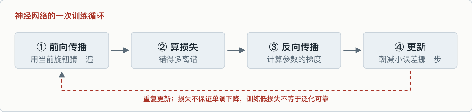
The size of the “small step” step is called the learning rate. If the steps are too large, they may fluctuate or even diverge; if too small, progress may be slow; In practice, training often uses learning rate scheduling rather than manually maintaining a single number.
Two parameters: Let the machine imitate its own rules
You can run the following code directly (numpy is required). We don’t tell the machine formulas, only four sets of data to see if it can find patterns on its own:
import numpy as np

# 我们心里的规律是 y = 3x + 2,但绝不告诉机器
x = np.array([1, 2, 3, 4], dtype=float)
y = np.array([5, 8, 11, 14], dtype=float)

w, b = 0.0, 0.0                    # 两个“旋钮”,初始值随便给
lr = 0.01                          # 学习率:每次拧多小的一步

for step in range(2000):
    pred = w * x + b               # ① 前向:用当前旋钮猜一遍
    error = pred - y               # ② 错了多少
    loss = (error ** 2).mean()     # ③ 损失:误差的平均平方

    grad_w = (2 * error * x).mean()   # ④ 反向:w 对这次错误负多少责任
    grad_b = (2 * error).mean()       #    b 负多少责任

    w, b = w - lr * grad_w, b - lr * grad_b   # ⑤ 两个旋钮各朝减小损失的方向挪一小步

    if step % 500 == 0:
        print(f"第{step}步 损失={loss:.4f} w={w:.3f} b={b:.3f}")

print(f"机器自己找到的规律:y = {w:.2f}x + {b:.2f}")**
The output of the knowledge base records in September 2026 is as follows: no retraining of the local large model was made this round:
第0步 损失=101.5000 w=0.550 b=0.190
第500步 损失=0.0064 w=3.066 b=1.805
第1000步 损失=0.0003 w=3.015 b=1.956
第1500步 损失=0.0000 w=3.003 b=1.990
机器自己找到的规律:y = 3.00x + 2.00
**Keep an eye on the second column. ** The loss dropped from 101.5 all the way to near zero, while knobs w and b climbed to around 3 and 2. No one told it the answer was 3 and 2; it was determined step by step by “moving the way the error minimized.”
Don’t believe the phrase “it found it on its own”—this is our first manual calculation update. The four sets of data are x = 1, 2, 3, 4, corresponding to y = 5, 8, 11, 14, with the prediction formula w×x + b. Initially, w = b = 0, all four predictions are 0; The average squared error is (25 + 64 + 121 + 196) ÷4 = 101.5.
Why use squares? If the two errors are +2 and −2, directly averaging will yield 0, which seems correct; After squaring, the average is 4, so the error will not cancel out the problem. Loss is not the only optional function, but it must match the task you want to solve.
| First update | The result | What does it say? |
|---|---|---|
| Gradient for w | −55 | Increasing W has the opportunity to reduce current losses |
| The gradient for b | −19 | Increasing B offers a chance to reduce current losses |
| Learning rate after 0.01 | w=0.55, b=0.19 | The old value minus the learning rate multiplied by the gradient |
| A new prediction of x=1 | 0.74, target 5 | A step in the right direction, but the study is not yet complete |
This table is not a newly tested large model; it is directly calculated from the previous four sets of data and code formulas. It also shows that gradients are not “error responsibility assigned to a certain proportion of parameters.” It is the local sensitivity of loss to parameter changes; both units and magnitudes depend on the data and objectives. Translating analogies back into formulas prevents the mathematical process from being mistaken for reflection.
Try changing another number. Change the learning rate lr from 0.01 to 0.001: After completing two thousand steps, it still stops halfway through w=3.16 and b=1.52. Change to 0.13: loss increases instead of decreases. Step 10 is 2386, step 100 is already 5 times 10 to the power of 15—the step is too big, each step crosses the lowest point, and the distance keeps increasing. Even more surprising, 0.11 converges faster than 0.01: for these four sets of data, the safety line is around 0.12, and once it crosses, the difference from fastest to losing control.
This code retains the framework of “forward computation→ loss→ gradient → updates,” but it is linear regression, not a full deep network or GPT. Actual training also involves handling architecture, morphology, batches, optimizer states, numerical precision, distributed communication, and data quality, and cannot be derived from cost or capability based solely on parameter multiples.
There is another more important question than the loss reduction: can the laws of the world really be determined by just these four points? A line 3x+2 can pass through them; Another equation, 3x+2+(x−1)(x−2)(x−3)(x−4), can pass through the same four points, because the product is zero at the training point.
At x=5, the first item is 17, the second is 41. The training data is exactly the same, the error at the training points is zero, but the unseen points differ by 24. This is a handcrafted counterexample; it doesn’t mean the actual model will choose the second one; It only proves that “the training problem is done” is not enough to deduce “the new problem will also be done.” Model structure, data range, and independent testing are precisely designed to solve this problem.
It’s like memorizing only a few routes you’ve practiced during a driving test: you get every intersection on a familiar road correctly, but switching to another route may not make a judgment. Overfitting means the model overly fits the details of the training materials, while generalization means whether you can still do well with materials you’ve never seen before. The validation data you set aside is used for selection settings, and the final test data is best avoided for such choices; If you repeatedly change answers based on “unseen” questions, those questions are actually helping you prepare for the test, and the value of independent checks decreases.
Why is it called “deep” learning?
Arranging neurons in one layer and stacking multiple layers together is called a deep neural network. “Depth” refers to having many layers.
What does the number of layers bring? Layer by layer abstraction. Take image recognition as an example: the first layer might only recognize edges and light and shadow; the second layer combines edges into textures and corner points; the third layer combines parts like eyes and wheels; and beyond that are concepts like “cat” and “car.”
With appropriate tasks and training, multi-layer networks can learn to gradually combine representations without needing to specify “this layer is responsible for the eyes” layer by layer. This example of image features helps understand that not every network follows a fixed division of labor table. Traditional machine learning also learns parameters and partial representations; The difference between the two cannot be simplified to relying entirely on humans before and now relying entirely on machines.
The cost is here: the intermediate representations machines learn are often unreadable; we know they work, but it’s hard to clearly define what each number represents. This is the so-called black box problem.
**What does this have to do with reviews? ** The “7B” and “27B” in the model names count the model’s parameters. They are the most prominent numbers on the model card, but not a measure of ability: with the same 27 billion knobs, different books and training methods can make the difference in skill very different (model scale and selection content later). For your computer, the first thing it decides is another thing—Can it fit it: Each knob takes up memory; the more knobs, the larger the file size (Hardware content in Issue 16).
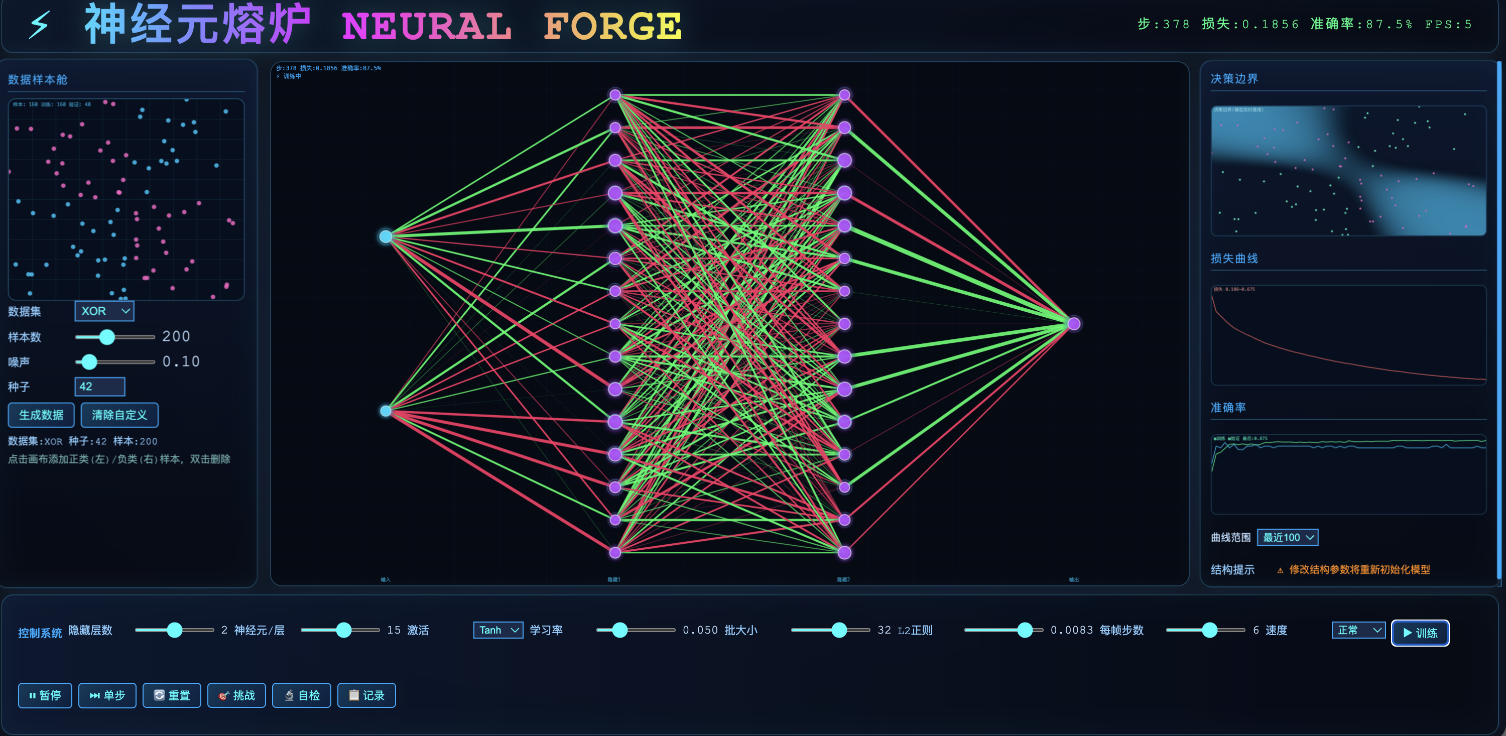
The screenshot shows an 87.5% accuracy rate, so why can’t it be declared a master?
The neuron melting pot interface left over from five questions in September shows 378 steps, loss 0.1856, accuracy 87.5%, and the interface also shows decision boundaries and curves. This is the state of that frame at that time, not the current re-measured result. What samples are involved in accuracy, whether there is an independent test set, how noise and seed are set, all change its meaning. No errors on the webpage, descending curve, and reliable generalization are three different things.
When reading this interface, first look at the decision boundary and sample, then read the accuracy. Which points does the boundary divide into two categories? Are scores from training samples or from reserved samples? If you keep changing settings while checking validation scores, the validation set will gradually participate in selection, and ideally, there will be a batch of test data that wasn’t used for picking settings.
This old screenshot doesn’t answer all the criteria for us, so 87.5% can only be interpreted based on the records at the time, not rewritten as “model has 87.5% intelligence.” Also, don’t attribute the classification score from the demo network to the language model that generated the webpage. One is responsible for being displayed, the other is responsible for writing the program; the evaluation targets are different.
| A common saying | Why is it easy to believe? | How to verify this |
|---|---|---|
| Reducing losses to zero is what you learn | The curve descent is very intuitive | Samples that did not participate in training were kept separately to check whether they only remembered the training points |
| The more chats you have, the smarter the model is | It can cite the previous answer | Distinguish between context changes, external memory writes, and weight updates |
| More specs mean stronger performance | The number of knobs resembles a capability scale | Control tasks, training data, and evaluation conditions—don’t just compare parameters |
With this in mind, I’ll give it a try
Just read the code, no need to start the large model: mark prediction, loss, gradient, and parameter updates in four areas; divide the learning rate comparison records into “convergence but slow,” “convergence faster,” and “divergence.” Then write two additional acceptance tests for the neuron furnace: independent sample performance and stability after seed switching. The safety threshold 0.1198 only belongs to these four sets of data and this update method from the original records; it cannot be used to adjust all neural networks.
Now you can answer the beginning: reduced loss means the calculated results for the selected data and objectives better meet training requirements; To say you learned the transferability pattern, you need to check with new examples that didn’t participate in training. The number of knobs, whether they were updated during training, and whether chats were carried into history must also be checked separately.
Several terms that appear in the story
| Terminology | Plain speech |
|---|---|
| Weight | Adjustable knobs to save learned parameters; External data and session status are not included |
| Bias | Each neuron is additionally given a fixed number to give it a base tendency |
| Activation function | Introduce nonlinear cornering actions; ReLU = negative number becomes 0 |
| Forward propagation | Use the current knob to calculate once and guess the guess |
| loss | A single number shows how outrageous this mistake was |
| Gradient gradient | The sensitivity and magnitude of loss to parameter changes; Not the proportion of responsibility |
| Backspread | Applying chain rules to find gradients along computational graphs; In 1986, a classic paper promoted multi-layer network training |
| Gradient descent | Step by step, move in the direction of reducing losses |
| Learning rate | How much should each step be moved? Too large a oscillation, too small and too slow |
| Parameter count | Total number of knobs. “7B” means seven billion knobs |
| The black box issue | The middle indicates unreadability, knowing the effect but not the reason |
Next article: The strawberry is still the same strawberry, with an extra space at the front, but the machine sees a different number of blocks. An old method from data compression—how to get into the chat window and change your cost, speed, and context?
References
Self-made software
Versions, changes and supported installers all come from the same public release records.
LocalBrain
Turn your Mac into a private AI toolbox for transcription, speech, images, video and MCP tools.
View public downloads and updates ↗HyphenBox
A free model API radar and local router, with ongoing availability checks and keys kept on your device.
View public downloads and updates ↗ScreenLex
Turn subtitles from your own films and shows into an English vocabulary library, entirely offline.
View public downloads and updates ↗HyphenScreen
Screen recording and editing with a Resolve-style timeline, automatic redaction and pre-export checks.
View public downloads and updates ↗Late nights and burned API credits went in,a cup of tea comes back out — only if you feel like it.
Scan with WeChatPress and hold to save the image, then open it from your album in WeChat Scan




Comments
Loading comments…